
4. Product Understanding#
4.1. Amount requested vs amount spent#
We evaluate retailers request for a given amount, but allow them to spend only a fraction of it. This means there are 2 related but distinct behaviors to capture: the rationale when requesting funds, and the actual need to spend them. I predict that there is a considerable delta between the 2: retailers overestimate their needs for funds but then quickly realize they won’t need as much. Let’s check if this prediction is valid by looking at how the delta is distributed.
Note
This “request loan but only pay for what you spend” functionality is quite appealing and likely to be a big source of engagement with the product. The trade-off being that it’s considerably harder to estimate our cash flow and liquidity. As the amount allocated to a given retailer cannot be made available to others (otherwise our liquidity can suffer), we run the risk of creating pools of stale capital that yields no margins.
It’s the growth versus profit conundrum. And I believe a good risk assessment and control engine must provide the ability to tweak its nobs to favor one or the other side.
Show code cell source
import pandas as pd
import matplotlib.pyplot as plt

try:
    _ = loans_df
except NameError:
    loans_df = pd.read_excel("../../data/Loans_Data.xlsx")

delta = (loans_df["SPENT"] / loans_df["LOAN_AMOUNT"])

fig, (ax1, ax2) = plt.subplots(1, 2, figsize=(15, 5))
_ = delta.plot.hist(
    bins=50,
    density=False,
    cumulative=False,
    log=True,
    ax=ax1
)
_ = delta.plot.hist(
    bins=50,
    density=True,
    cumulative=True,
    ax=ax2
)

_ = ax1.set_ylabel("Count of retailers (log scale)")
_ = ax1.set_xlabel("Percentage (bins)")
_ = ax1.set_title("What percentage do retailers actually spend?")

_ = ax2.set_ylabel("Cumulative probability")
_ = ax2.set_xlabel("Percentage (bins)")
_ = ax2.set_title("What percentage (bins) account for most observations?")
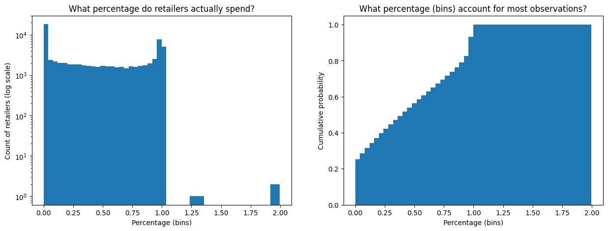
Well, this is unexpected. The plot above shows us that a large percentage of retailers spend nothing of LOAN_AMOUNT. However, more unexpected is that there are cases where the SPENT is greater than LOAN_AMOUNT. This could be data quality issues or product functionality that I’m unaware of. Let’s first get a better understanding of both scenarios.
Loans which retailers spend nothing#
What is the percentage of retailers that contract loans but spend nothing of it? Let’s look at the quantiles of the delta series:
Show code cell source
(loans_df["SPENT"] / loans_df["LOAN_AMOUNT"]).quantile(
    [.01, .1, .15, .20, .205, .21, .215, .225]
)
0.010    0.000000
0.100    0.000000
0.150    0.000000
0.200    0.000000
0.205    0.000000
0.210    0.000000
0.215    0.003269
0.225    0.011485
dtype: float64
This tells us that 21% of retailers that contract loans end up spending nothing of it. As I mentioned before, this seems to be counterproductive for us but understandable behavior because acquiring the loan is free and retailers must only pay for what they spend. It could also just be an artifact of retailers testing out the new functionality. But we wouldn’t want to encourage it.
Now, let’s look at the second, and more puzzling, case.
Loans which retailers spend more than borrowed#
Section conclusion
You’ll see that after investigation in this section, I have better understanding of the product and realize “loans where retailers spend more than borrowed” is a non-issue.
Let’s first uncover how frequently this happens in this dataset. We start by inspecting the history of loans of a retailer that shows this behavior.
Show code cell source
(
    loans_df[(loans_df["SPENT"] / loans_df["LOAN_AMOUNT"]) > 1]
    [[
        "MAIN_SYSTEM_ID",
        "LOAN_ID",
        "LOAN_AMOUNT",
        "SPENT"
    ]]
)
| MAIN_SYSTEM_ID | LOAN_ID | LOAN_AMOUNT | SPENT | |
|---|---|---|---|---|
| 8702 | 83079 | 706927 | 3000.00 | 3863.15 |
| 15567 | 50527 | 4917 | 3000.00 | 3750.19 |
| 36742 | 71029 | 951366 | 2000.00 | 3991.98 |
| 57057 | 66104 | 899831 | 1000.00 | 1927.43 |
| 57812 | 56822 | 695593 | 548.81 | 729.96 |
| 66486 | 71029 | 951555 | 2000.00 | 3991.98 |
| 69473 | 66104 | 899779 | 1000.00 | 1927.43 |
Let’s investigate retailer MAIN_SYSTEM_ID == 83079. We’ll look at the first loans they requested.
Note
The following plot is transposed so that we can fit all data points of interest in the page. This means each loan becomes a column increasing left to right based on LOAN_ISSUANCE_DATE.
Show code cell source
(
    loans_df.query("MAIN_SYSTEM_ID == 83079")
    .sort_values("LOAN_ISSUANCE_DATE")
    .head(3)
    [[
        "MAIN_SYSTEM_ID",
        "LOAN_ID",
        "LOAN_ISSUANCE_DATE",
        "LOAN_AMOUNT",
        "SPENT",
        "PAYMENT_AMOUNT",
        "FIRST_TRIAL_BALANCE",
        "REPAYMENT_AMOUNT",
        "CUMMULATIVE_OUTSTANDING",
        "INITIAL_DATE",
        "REPAYMENT_UPDATED"
    ]]
    .T
)
| 69151 | 8702 | 41838 | |
|---|---|---|---|
| MAIN_SYSTEM_ID | 83079 | 83079 | 83079 |
| LOAN_ID | 706905 | 706927 | 710622 |
| LOAN_ISSUANCE_DATE | 2022-09-04 12:07:14.473000 | 2022-09-04 12:14:34.304000 | 2022-09-05 14:32:47.728000 |
| LOAN_AMOUNT | 4000.0 | 3000.0 | 3000.0 |
| SPENT | 3863.15 | 3863.15 | 2039.41 |
| PAYMENT_AMOUNT | 4000.0 | 3000.0 | 3000.0 |
| FIRST_TRIAL_BALANCE | 136.85 | -3863.15 | 960.59 |
| REPAYMENT_AMOUNT | 0.0 | 4000.0 | 0.0 |
| CUMMULATIVE_OUTSTANDING | 136.85 | 136.85 | 960.59 |
| INITIAL_DATE | 2022-09-05 00:00:00 | 2022-09-05 00:00:00 | 2022-09-06 00:00:00 |
| REPAYMENT_UPDATED | 2022-09-05 11:29:54.764000 | 2022-09-05 11:29:54.764000 | 2022-09-06 12:17:39.343000 |
The first 2 loans (706905, 706927) seem to have been a confusion on the retailer’s side. They took 706927 7 minutes after 706905, paid both loans in the first collection attempt, but all ecommerce orders funded since LOAN_ISSUANCE_DATE were still due to be collected, thus the negative FIRST_TRIAL_BALANCE on the second loan 706927. They probably realized their mistake and added $4k as REPAYMENT_AMOUNT, which left $136.85 positive balance in their account represented by CUMMULATIVE_OUTSTANDING. So, this is not a good example for our investigation.
However, this leads me to understand that SPENT is not really tied to the loan itself, but starts being aggregated over all of the retailer’s ecommerce orders once the loan is issued. In other words, the retailer can use the loan as a top-up to fully fund their orders, which means they end up spending more than the loan itself. Thus, we can conclude this is not a problematic scenario after all.